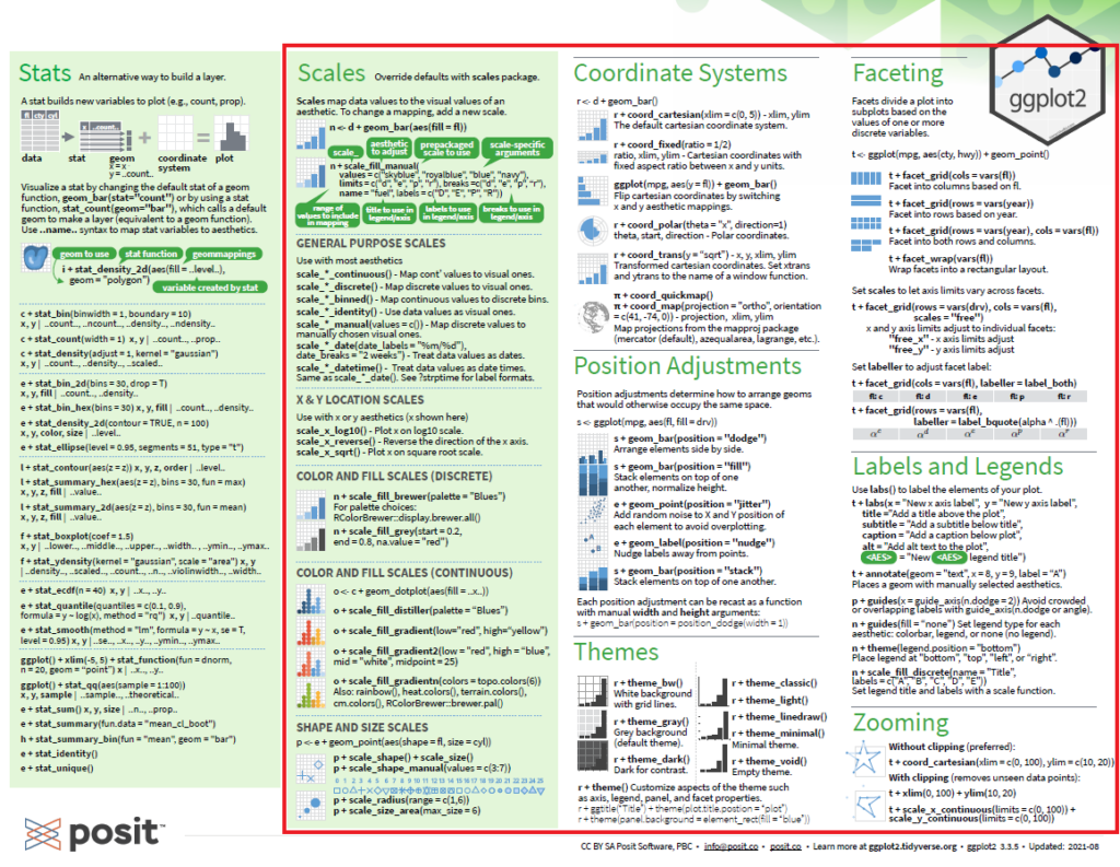
R cheat sheets were my go-to aid as a new-comer to R. These cheat sheets provide a quick overview of the essential commands within a specific package of R. However, the information can be hard to appreciate if one is not familiar with R or R language. Fellow newcomers to R have also reiterated similar thoughts concerning R cheat sheets. In this article, I will provide a simple introduction to the ggplot2 cheatsheet that will hopefully make the information in the ggplot2 cheatsheet more accessible to R new-comers.
Quick summary
- The ggplot() code is the main code for data visualisation with the ggplot2 package.
- The minimum requirements of the ggplot() code are a dataset, the aes() code, and a geom_ or stat_ function.
- The aes() code must contain information on the variable to be displayed on the x-axis, and the y-axis if applicable.
- The information under geoms and stats are displayed as geoms or stats added to an object. The object is a ggplot() code, and is specified under each subheading.
- Next to each example of a geom or stat, information are displayed describing the “aesthetics” or sub-codes that can be changed within the specific code.
Basics and geoms
This box introduces the ggplot() command. This is the essential command of the ggplot2 package as the qplot() command has been deprecated. The ggplot() command has subcommands that are required, and optional subcommands that allow customization.
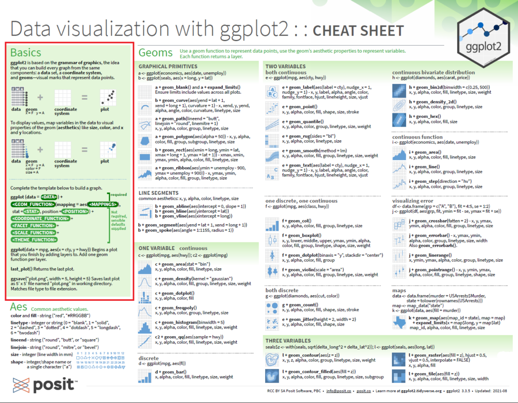
The required parts of the ggplot() command include:
- Data – which consists of a dataset.
- aes() – which must as a minimum include information on the variable to be displayed on the x-axis. If the graph displays information on more than one variable, then these are also specified here.
The box summarises this information in this line
ggplot(data = mpg, aes(x = cty, y = hwy)).
This command can be simplified to
ggplot(mpg, aes(cty, hwy))
Here, mpg is a dataset (mpg is an example dataset provided in the ggplot package). Cty and hwy are continuous variables within the dataset, and in the above code, cty is chosen to be displayed on the x-axis, while hwy is chosen to be displayed on the y-axis.
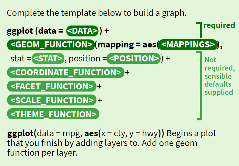
Now we can add a geom function to display the data. The geoms box provides information on the most commonly used geoms according to the appropriate number and type of data that these can represent. For example we can add geom_point().
The code will be:
ggplot(mpg, aes(cty, hwy)) + geom_point()
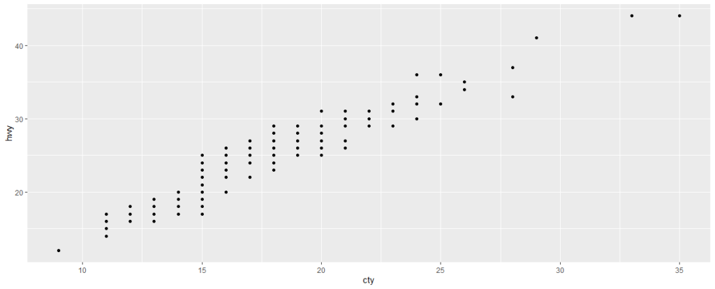
The ggplot cheat sheet shows examples of many geoms. To simplify the code of these, the ggplot() command has been saved as an object. For example:
e <- ggplot(mpg, aes(cty, hwy))
Now “e” is an object that means “ggplot(mpg, aes(cty, hwy))”. Instead of repeating the ggplot command for each graph, we can add geoms by writing:
e + geom_point()
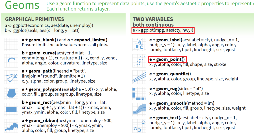
Several geoms can be added to the same ggplot command:
e + geom_point() + geom_smooth()
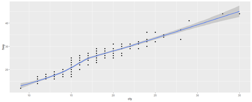
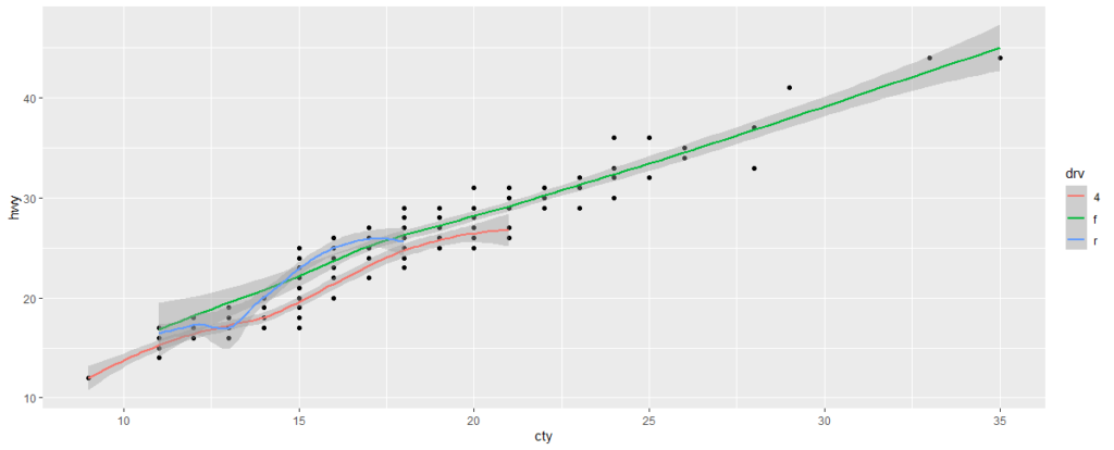
Each geom can be customised with sub-commands or “aesthetics”. These are listed next to each geom in the ggplot cheat sheet. These aesthetics can be specified in the ggplot command, if one wants these specifications to apply for all geoms specified after the ggplot command.
ggplot(mpg, aes(cty, hwy, color = drv))+
geom_point()+
geom_smooth()
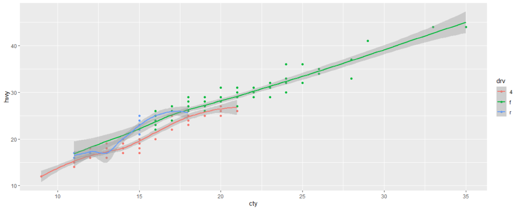
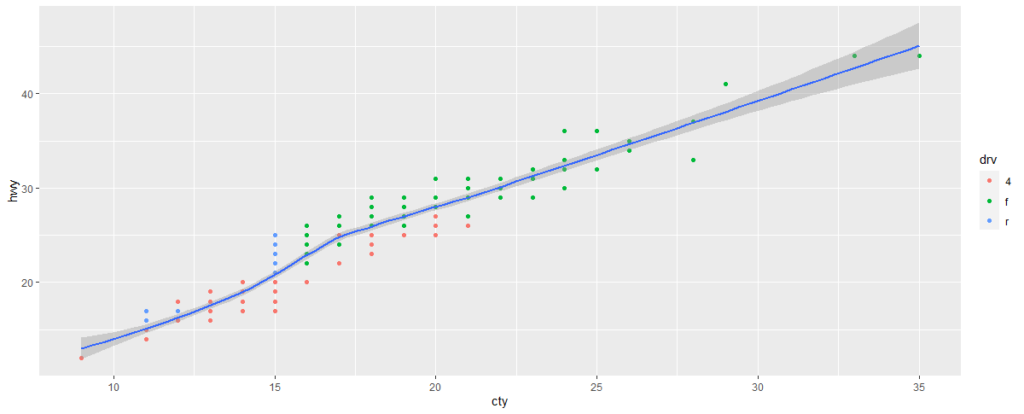
If one wants the customization to apply to only one layer, these specifications should be put in the specific geom.
ggplot(mpg, aes(cty, hwy))+
geom_point(aes(color = drv))+
geom_smooth()
ggplot(mpg, aes(cty, hwy))+
geom_point()+
geom_smooth(aes(color = drv))
Stats
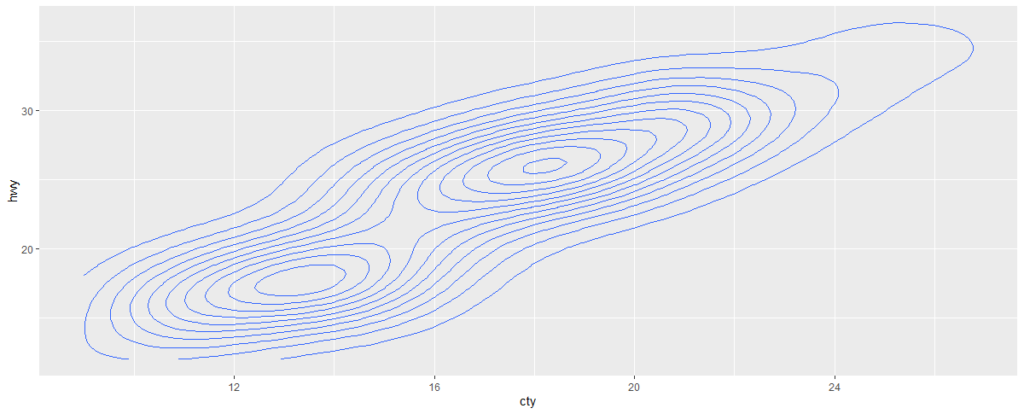
Stats are an alternative way to build graphs. The stat codes perform statistical transformation of the data and displays them in a graph.

e + stat_density2d(contour = T, n = 100)
According to R documentation, stat_density2d() performs a 2D kernel density estimation and displays the results using with contours.
Customization
The information of the ggplot2 cheat sheet so far is sufficient for generation of a wide variety of basic graphs. The rest of the cheat sheet deals with customization. As the information geoms, the information in this part of the cheat sheet is displays as additions to a ggplot code.
